Rise and fall of the German economy.

The number of Germany’s corporate insolvencies in March reached the highest level on record, new data reveal. It’s the Great Green Energies economic debacleBlackout News here calls the trend “alarming” and that it is “a clear sign of the worsening economic crisis. The news are based on data released by the Halle Institute for Economic Research (IWH).

link to Pierre L Gosselins recent post.

Rise And Fall Of The German Economy… Energy Debacle Leading To Economic Meltdown

The North Atlantic Ocean Is in a State of Reduced Overturning

In previous Article presented here we took a look at the AMOC (Atlantic Meridional Overturning Circulation) on data sets available.
Carrying on from this we now have supporting evidence to suggest a slowdown and shift in this pattern.

Geophysical Research Letters Volume 45, Issue 3
Research Letter Open Access
The North Atlantic Ocean Is in a State of Reduced Overturning
D. A. Smeed S. A. Josey C. Beaulieu W. E. Johns B. I. Moat … See all authors
First published: 29 January 2018
https://doi.org/10.1002/2017GL076350
Cited by: 2
About
Sections

Abstract
The Atlantic Meridional Overturning Circulation (AMOC) is responsible for a variable and climatically important northward transport of heat. Using data from an array of instruments that span the Atlantic at 26°N, we show that the AMOC has been in a state of reduced overturning since 2008 as compared to 2004–2008. This change of AMOC state is concurrent with other changes in the North Atlantic such as a northward shift and broadening of the Gulf Stream and altered patterns of heat content and sea surface temperature. These changes resemble the response to a declining AMOC predicted by coupled climate models.
Link
https://agupubs.onlinelibrary.wiley.com/doi/full/10.1002/2017GL076350

Ocean/Atmospheric coupling.

For many years AGW (Anthropogenic Global Warming)has been forced down the throats of humankind, understandably many have joined the gravy train.
As Oceans contain the greatest percentage of ALL CO2 on this planet, retention and distribution is often overlooked by the AGW “CLSN”,vast temperature swings ARE associated with ocean currents,

An article I came across in Britannica explains in detail how this function operates..link below.

https://www.britannica.com/science/climate-meteorology/Temperature

Valentina Zharkova (Wave amplitude)

Today we  review and take a look at the Wave Amplitude graph produced by Prof Valentina Zharkova and her team of Scientists.

Zharkova

First we look at the graph and see “the medieval warm period” dated as 1400-1530 approx, there are several dates given for the Medieval warm period 950-1250, 800-1400 seem to be the years cited by many outlets, the above suggests 1350-1530? I see no connection to the MWP around these dates. However we did see a peak in temps around 1500 + 1720 during the colder period after the medieval optimum, LIA, see below.

nmnmnm

This peak is visible in the Zharkova graph (G1) but does not depict the MWP. We then see from the graph (G2) another peak around 1720 that does not fit in the graph of Zharkova in (G1), as these peaks were of similar strength (1500+1720) expectations would be; the Dynamic strength of the Wave Amplitude should be similar in (G1), they are not, peak in 1900 fits the Zharkova graph modern Maxima (G1+G2).

The wave Amplitude in (G1) “reduction in wave amplitude” fits the Maunder Minimum of 1645-1715 above, However the Dalton event of solar cycle 4-7 does not fit (1790-1830 or 1796-1820).

Let us take a look at the Graph with all the details i have overlaid below. (G3)

zharkova

Note the Maunder does fit, however the wave amplitude suggests weaker cycles from 1715-1770, 40 years prior to the Dalton. Overlaying the solar cycles onto the Wave Amp graph indeed does suggest cycle 25 will be the start of the Eddy Minimum lasting at least 5-6 cycles before an increase in wave Amplitude around 2100 however does not suggest a second Amplitude crossover (cancel out) as we seen during the late 1700’s, solar cycle 25 will be a positive magnetic polar north.

Looking at the cycle progression (sunspot graphs) we can also see that there is no obvious connection in wave amplitude and strength of the cycle, as 3/4/8/9/11/18/19/21 cycles were the strongest cycles, however (G1) suggests 3/4/8/19 were not the strongest in wave amplitude.

We should not therefore associate sunspot groupings or cycle magnitude with the “WAVE AMPLITUDE” as this is a very poor fit, However there is an obvious long term correlation to a weak and strong wave Amplification over the last 700 years of reconstructed observations, that show cyclic behaviour of the Toroidal and Magnetic fields, moreover the reconstruction suggests a “cancellation” around solar cycle 26 commencement around 2030 (± 3 years), although there is some differences in Dates within (G1) it does not take away from the overall progression of reconstructed wave Amplification which could take place at cycle 25/26 leading to a significant reduction in Plasma density, speed and dynamic pressure leaving the corona, resulting in significant reductions in land and sea temperatures. Of course as with every reconstructed scientific theorems we need to see the results play out, if indeed they do then this is a major leap forward in the understanding of solar cycles and magnetohydrodynamics, we must also correlate Land and Sea temperatures to this theory also as the connection must be valid with all the other feedbacks of  solar activity, Sunspots, Plasma wind density, speed, Proton Flux, F10.7cm flux, Coronal mass ejections, flares etc must all be connected to the Wave Amplitude.

Growing food “The Russian Way”

During times of low solar activity heading into a new era of Global cooling one should seek the very best information with regards to survival, we all need sustenance to energies our metabolism and go about the “recovery” period.

 Millions of Russians commute to rural dacha gardens from May to September. While some Russians do have a garden by their primary home (ogoro), many more commute an hour or more to reach the family’s dacha garden.Working with an average space of 6 sotkas (600 square metres, or about 6458 square feet) and a growing seasons of less than 120 days north of Moscow, Russian dacha gardeners (dachniks) provide half of Russia’s food supply by working hard, making the most of what they have, and generously sharing the bounty with one another.

The following article Written by Barbara Pleasant Takes us through the several very interesting methods used, inclusive is a small video actually taken in a dacha Garden.

Lets go to the dacha

THE DAWNING OF MODERN MINIMA BY THE YEAR 2035/40

It is known that the Sun has its own magnetic field, the amplitude and spatial configuration of which vary with time. The formation and decay of strong magnetic fields in the solar atmosphere results in the changes of electromagnetic radiation from the Sun, the intensity of plasma flows coming from the Sun, and the number of sunspots on the Sun’s surface. study of changes in the number of sunspots on the Sun’s surface has a cyclic structure vary in every 11 years that is also imposed on the Earth environment as the analysis of carbon-14, beryllium-10 and other isotopes in glaciers and in the trees showed.

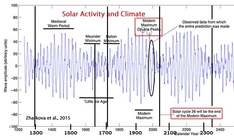
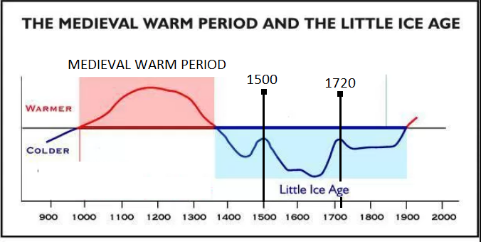
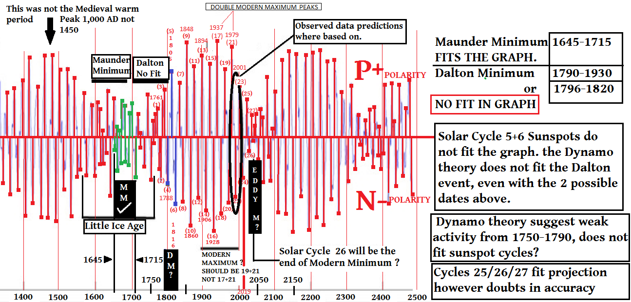
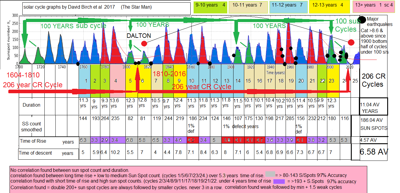
There are several cycles with different periods and properties, while the 11-year cycle, the 206-year cycles are the best known of them. The 11-year cycle appears as a cyclical reduction in stains on the surface of the Sun every 11 years. Its 206-year variation is associated with periodic reduction in the number of spots in the 11-year cycle in the 60-70%. during the 17th century there was a prolonged reduction in solar activity called the Maunder minimum, which lasted roughly from 1645 to 1715. During this period, counts of only about 50 sunspots instead of the usual 40-50 thousand sunspots where observed. Analysis of solar radiation showed that its maxima and minima coincided with the maxima and minima in the number of spots.

solar cycles ORIGINAL DOC

Researchers have analysed a total background magnetic field from full disk magnetograms for three cycles of solar activity (21-23) by applying the so-called “principal component analysis”, which allows to reduce the data dimensionality and noise also to identify waves with the largest contribution to the observational data. This method can be compared with the decomposition of white light on the rainbow prism detecting the waves of different frequencies. As a result, the researchers developed a new method of analysis, which helped to uncover that the magnetic waves in the Sun which proved to have been generated in pairs, with the main pair covering 40% of variance of the data (Zharkova et al, 2012, MNRAS). The principal component pair is responsible for the variations of a dipole field of the Sun, which changes its polarity from pole to pole (N>S) during 11-year solar cycle.

These magnetic waves travel from the opposite hemisphere to the Northern Hemisphere (odd cycles) or to Southern Hemisphere (even cycles), with the phase shift between the waves increasing with a cycle number. These waves interact with each other in the hemisphere where they have maximum (Northern for odd cycles and Southern for even ones). These two components are assumed to originate in two different layers in the solar interior (inner and outer) with close, but not equal, frequencies and a variable phase shift (Dr. Helen Popova of the Skobeltsyn Institute of Nuclear Physics).

The scientists lead by Zharkova managed to derive the analytical formula, correlating the evolution of these two waves and calculated the summary curve which was linked to the variations of sunspot numbers. The scientists made the first prediction of magnetic activity in the cycle 24, which gave 97% accuracy in comparison with the principal components derived from the observations. They then extended the prediction of these two magnetic waves to the next two cycles 25/26 and discovered that the waves become fully separated into the opposite hemispheres in cycle 26 and thus have little chance of interacting and producing sunspot numbers. This will lead to a sharp decline in solar activity in years 2035—2040 comparable with the conditions existed previously during the Maunder minimum in the 17th century when there were only 50-70 sunspots observed instead of the usual 40-50 thousand expected.

The stage is then set for this to result in a reduction of solar irradiance of 3wm², this reduction will result in severe cold winters and shortened growing seasons across the United states Asia and eastern Europe. Dr Helen Popova says “Waters in the river Thames and the Danube will freeze over, the Moscow river will freeze every six months and snow will lay on the some plains all year round”. Greenland will revert back to full glaciation.

The study of deuterium in the Antarctic showed that there were five global warmings and four Ice Ages for the past 400 thousand years. Increases in the volcanic activity comes after an Ice Age this then leads to the greenhouse gas emissions. The magnetic field of the Sun grows, which means that the flux of cosmic rays decreases, decreasing the number of clouds and leading to the warming again. Next comes the reverse process, where the magnetic field of the Sun decreases, the intensity of cosmic ray rises, increasing the cloud nucleation and making the atmosphere cool again. However this process does come with some delay.

On closing There is no strong evidence, that global warming is caused by human activity. The study of deuterium in the Antarctic showed that there were five global warmings and four Ice Ages in the past 400 thousand years. People first appeared on the Earth about 60 thousand years ago, CO2 levels have been much higher than “modern eras” so the conclusion that “man made” Anthropogenic warming is unfortunately driven by political agenda and fundamentally flawed.

F10.7cm Flux Trends. A new era?

My Research and observations into the progression of F10.7cm solar flux have resulted in the following conclusions.

SUNSPOTS VS 10.7CM FLUX

1-Cycle minimum of October 1964 the 10.7cm flux took 21 months to get above 100.(add decimal point in graph). 106.7 july 1966.
high solar flux then lasted 83 months =6.9yrs to may 1973.
2.-June 1973-November 1977 low solar Flux. 53 months =4.4yrs.
3- December 1977-June 1984 High solar flux. 70 months = 5.8yrs.
4. July 1984 – Jan 1988 Low solar Flux
41months = 3.4yrs.
5-Feb 1988 – June 1993 High solar Flux
64 months = 5.3yrs.
6-July 1993 – March 1998 Low solar Flux 58months. = 4.8yrs
7-April 1998 – November 2004 High solar Flux 89 months. = 7.4yrs.
8-December 2004 – March 2011 Low solar Flux
70 months = 5.8yrs.
9- April 2011 – February 2016 High solar flux
58months = 4.8yrs.
10- March 2016 – Current low solar flux, = 21 months this on trend will continue for at least the next 35/40 months or 2.9/3.3yrs. = Sept 2020/ March 2021. excluding intermittent short F10.7 months as in September 2017 x-class Flares.
The Overall conclusion is that F10.7cm Flux has a negative trend in time scale from April 1998 when the highest period length of F10.7 lasted 7.4 years.
F10.7 flux is our guide to energy emitted from the Sun, this negative trend suggests a deep Minimum in the coming decades with trending long term low 10.7cm flux.

This will result in a reduction of Solar Irradiance and an overall downward trend in Temperatures; as we are already seeing from the Teleconnections during 2016/17 in the Northern Hemisphere.